beamax
![]()
![]()
Install | Examples | API reference
beamax is a JAX library for solving photoacoustic tomography problems using the multiscale Gaussian beam method.
Installation
Python 3.11 or 3.12 is required.
- Install JAX for your hardware (CPU/GPU/TPU) following the official instructions.
- Install
beamax:
Optional extras:
# With matplotlib examples
pip install "beamax[viz-mpl]"

# With k-Wave integration
pip install "beamax[kwave]"
For development, see CONTRIBUTING.md.
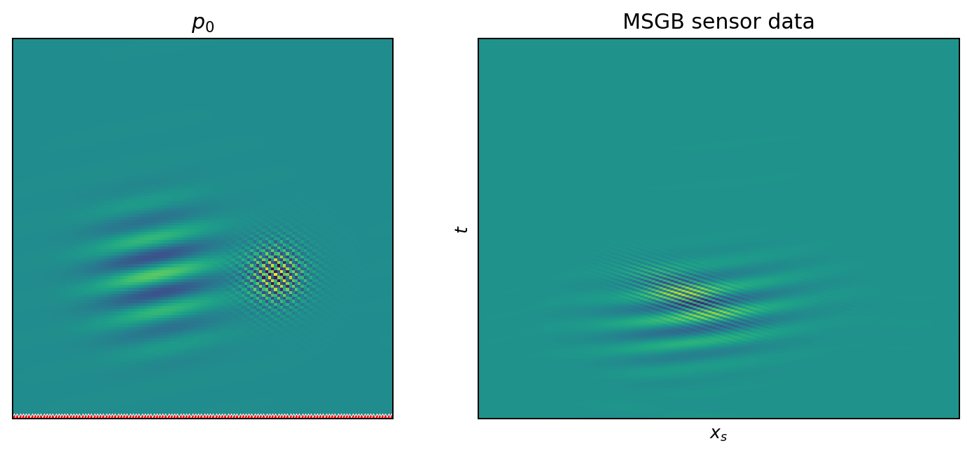
Example
This example runs a small 2D photoacoustic forward solve. A high-frequency \(p_0\) is propagated to a planar detector with MSGB.
import jax
import jax.numpy as jnp
import matplotlib.pyplot as plt
import numpy as np

from beamax import Domain, Sensor, DyadicDecomposition, MSWPT
from beamax import transforms, utils
from beamax.gb import gb_solvers
from beamax.solvers import MSGBSolver

# Use double precision for this small MSGB example.
jax.config.update("jax_enable_x64", True)


# Build the same two-packet $p_0$ used by examples/forward/2d_forward.py.
def make_initial_pressure(dyadic):
    grid = dyadic.fourier_meshgrid
    high = transforms.compute_frames(
        dyadic,
        125,
        jnp.array([11, 6]),
        grid,
        redundancy=2,
        windowing="none",
    )
    low = transforms.compute_frames(
        dyadic,
        44,
        jnp.array([11, 3]),
        grid,
        redundancy=2,
        windowing="none",
    )

    p0 = utils.unitary_ifft(high) + utils.unitary_ifft(low)
    p0 = p0 / jnp.max(jnp.abs(p0))
    return p0.T.real


# 1. Define a 128 x 128 PAT domain with homogeneous sound speed.
n = (128, 128)
domain = Domain(
    N=n,
    dx=(1.0e-4, 1.0e-4),
    c=1500.0,
    cfl=0.3,
    periodic=(False, False),
)

# 2. Build the multiscale wave-packet transform and $p_0$.
decomp = DyadicDecomposition(
    num_levels=3,
    N=domain.N,
    num_boxes_levels=(4, 8, 16),
    box_aspect_ratio=(1, 1),
)
wpt = MSWPT(decomp, redundancy=2, windowing="rectangular_mirror")
p0 = make_initial_pressure(decomp)

# 3. Choose a time grid and put a one-sided detector line on the lower boundary.
ts = domain.generate_time_domain()
sensor_mask = jnp.zeros(n).at[0, :].set(1.0)
sensors = Sensor(domain=domain, binary_mask=sensor_mask)

# 4. Configure the MSGB forward solver and keep 4096 beams.
solver = MSGBSolver(
    thr=4096,
    thr_strat="top_n",
    batch_size=128,
    input_type="spatial",
    ode_solver=gb_solvers.solve_hom_diag,
    sum_method="scan_real",
)

# 5. Apply the MSGB forward operator: $p_0$ -> sensor data.
msgb_data = solver.forward(p0, domain, sensors, ts, wpt)
msgb_data = np.asarray(msgb_data.block_until_ready())

# 6. Plot $p_0$ and MSGB sensor data.
fig, axes = plt.subplots(1, 2, figsize=(8, 3.5), constrained_layout=True)
axes[0].imshow(np.asarray(p0), origin="lower", cmap="viridis")
sensor_rows, sensor_cols = np.nonzero(np.asarray(sensor_mask))
axes[0].scatter(
    sensor_cols,
    sensor_rows,
    marker="^",
    c="red",
    s=18,
    edgecolors="white",
    linewidths=0.4,
)
axes[0].set_title(r"$p_0$")
axes[0].set_xticks([])
axes[0].set_yticks([])
axes[1].imshow(msgb_data, origin="lower", aspect="auto", cmap="viridis")
axes[1].set_title("MSGB sensor data")
axes[1].set_xlabel(r"$x_s$")
axes[1].set_ylabel(r"$t$")
axes[1].set_xticks([])
axes[1].set_yticks([])

plt.show()
This produces:
For a fuller k-Wave/MSGB/Hybrid comparison, see
examples/forward/2d_forward.py.
Running examples
The public examples are listed in the examples gallery. Several have Open in Colab links if you want to try them on a GPU or TPU runtime.
From a local checkout, for example:
Example figures are written under plots/<category>/, matching the script's
directory under examples/.
References
beamax's MSWPT/MSGB implementation follows:
- Jianliang Qian and Lexing Ying, "Fast Multiscale Gaussian Wavepacket Transforms and Multiscale Gaussian Beams for the Wave Equation", Multiscale Modeling & Simulation, 8(5), 1803-1837, 2010.
Related Projects
Related acoustic simulation projects:
- k-Wave — MATLAB/C++ toolbox for time-domain acoustic and ultrasound simulations.
- k-Wave-python — Python wrapper used by beamax through the optional
[kwave]extra. - j-Wave — differentiable acoustic simulations in JAX.
License
MIT; see LICENSE.
Citation
If you use beamax, please cite this repository. If you use the MSWPT/MSGB method, also cite Qian and Ying (2010).